Example: a liquid bridge between two beads

A droplet wets two nearly touching spherical beads and forms a capillary bridge: the shape of minimal surface energy at fixed liquid volume, meeting each bead at a prescribed contact angle \(\theta\). Bridges like this hold wet granular media together; the force they exert depends on the gap between the beads and on \(\theta\).

This is the drop on a table of Getting started with two spheres for the table: contact angles on curved solids, the force between them, and a volume mesh of the liquid. It uses the conventions set out there, and relax() as in the tutorial.

The beads have radius 1 and the liquid–gas surface tension is 1, so lengths are in bead radii, energies in surface tension × radius², and forces in surface tension × radius. The adjustable parameters:

• theta: the contact angle in degrees, measured inside the liquid (below 90°: wetting);

• gap: the distance between the bead surfaces (0: touching);

• volume: the liquid volume.

import numpy as np
import matplotlib.pyplot as plt
import pyvista as pv
import pysurfaceevolver as pyse
from pysurfaceevolver import constraints as C

pv.set_jupyter_backend("static")    # "trame" in Jupyter for interactive views
pv.global_theme.window_size = [600, 450]

The model

Only the liquid–gas surface is made of facets. The beads are constraints: the two contact lines live on the spheres \(x^2 + y^2 + (z \pm c)^2 = 1\), with \(c = 1 + \mathrm{gap}/2\), and slide freely on them. The wetted part of each bead is not meshed; it enters as integrals along the contact line, which Evolver adds to the edges on a constraint (as in the mound.fe sample, there on a plane):

• Energy. Wetting a unit area of bead replaces solid–gas by solid–liquid surface, a change of \(\gamma_{SL} - \gamma_{SG} = -\cos\theta\) (Young’s law). So the energy is the liquid area plus \(-\cos\theta\) times the wetted area of each bead.

• Volume. Evolver computes a body’s volume from its facets as \(\int z\, n_z\, dA\); the wetted caps close the liquid’s boundary, so their part of that integral is added too.

pyse.constraints.sphere writes both integrals. Over the azimuth \(\phi\) about the \(z\) axis, with \(h\) the height above a bead’s centre, the wetted area is \(\oint R\,h\,d\phi\) up to the pole facing the gap (the integrand is singular at the poles), and the bead’s share of \(\int z\, n_z\, dA\) is \(\oint (c_z h^2/2 + h^3/3)\, d\phi\). Told which pole is wet (wet_poles), the builder knows what those integrals leave out: the volume over the pole, which it takes into the volume integral, and a constant energy \(-\cos\theta \cdot 2\pi R^2\) per bead, which ev.energy includes and Evolver’s own ev.total_energy leaves out (see Energies). It doesn’t change with the gap, so forces don’t see it. The contact angle is the datafile parameter theta and the bead centres follow the parameter gap (\(c\) = radius + gap/2 in the formulas), so both can be changed on a loaded surface.

def beads(radius=1.0):
    # the two beads, wetted around the poles that face each other; their
    # centres follow the datafile parameter gap, the contact angle theta
    return {1: C.sphere((0, 0, "-(radius + gap/2)"), radius, contact_angle="theta",
                        wet_poles=("north",)),
            2: C.sphere((0, 0, "radius + gap/2"), radius, contact_angle="theta",
                        wet_poles=("south",))}

def load_bridge(gap, theta, volume, radius=1.0, a=0.5):
    # a cylinder of liquid of radius a between the beads, its ends on the bead
    # surfaces (relaxing meets the volume); normals point out of the liquid
    zb = radius + gap/2 - np.sqrt(radius**2 - a**2)
    tube = pyse.shapes.tube(a, -zb, zb, nz=4, nt=12)
    ev = pyse.Evolver()
    ev.load_arrays(tube.vertices, tube.faces, constraints=beads(radius),
                   vertex_constraints={1: tube.rims["bottom"], 2: tube.rims["top"]},
                   bodies=[pyse.Body(volume=volume)],      # volconst: from the beads
                   parameters={"radius": radius, "gap": gap, "theta": theta})
    return ev

Relaxing

ev.relax(levels=3) refines the mesh three times (to about 6000 facets), with gradient steps in between, and ends with Newton steps. Every ten steps it equiangulates and averages vertices: without that, facets at the contact line get thin and collapse when the contact line moves. On the coarse starting mesh the contact line can still collapse within a few steps; relax() notices the jump in the residual, undoes those steps and moves on (Relaxing a surface has the details).

Very low contact angles at larger gaps make the contact line travel far over the beads; there the bridge is relaxed at 40° first and theta is then lowered in steps of 10°, relaxing after each.

def liquid_bridge(gap=0.2, theta=40.0, volume=0.3, callback=None):
    ev = load_bridge(gap, max(theta, 40.0), volume)
    ev.relax(levels=3, callback=callback, every=10)
    while ev.parameters["theta"] > theta + 1e-9:
        ev.parameters["theta"] = max(theta, ev.parameters["theta"] - 10)
        ev.relax()
    return ev

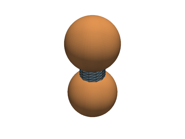
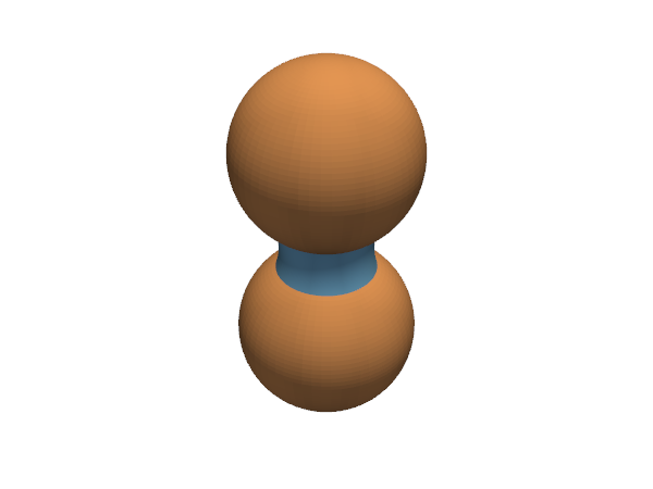
Here is a bridge relaxing from its starting cylinder. In Jupyter (trame backend) the live view redraws during the run; these docs show its first frame, and the relaxed bridge below.

gap, theta, volume = 0.2, 40.0, 0.3

ev = load_bridge(gap, theta, volume)
view = ev.live_view(color="lightskyblue", opacity=0.9, walls=True)   # the beads too
view.plotter.camera_position = [(3.2, -3.2, 1.2), (0, 0, 0), (0, 0, 1)]
ev.relax(levels=3, callback=view.update, every=10);

ev.plot(color="lightskyblue", smooth_shading=True, show_edges=False, walls=True)
ev

Evolver

datafile	surface.fe
model	soapfilm, linear
elements	3,168 vertices · 9,312 edges · 6,144 facets · 1 body
energy	9.81198012
area	1.79211847
threads	1 · solver evolver

Bodies

body	volume	target	pressure
1	0.3	0.3	0.8131985888	fixed

Checking the result

The contact angle is not imposed on the mesh: it comes out of the energy balance at the contact line. Measuring it is a check of the whole model: at each contact-line vertex, the angle between the liquid surface’s normal (out of the liquid) and the bead’s outward normal.

The pressure is the Lagrange multiplier of the volume constraint. The force between the beads follows from the neck, the narrowest circle in the mid-plane: there the surface is vertical by symmetry, so the force transmitted through that plane is \(F = 2\pi r_n \gamma - \pi r_n^2\, \Delta p\) (positive: the beads attract). It must also equal the change of energy with the gap at fixed volume, \(F = dE/d\,\mathrm{gap}\), here from bridges built at the gap plus and minus 0.01 (ev.derivative(name) does this for a parameter the constraint formulas use; the bead centres are numbers in them).

def neck_radius(ev):
    # mean radius where the liquid surface crosses the mid-plane z = 0
    ring = ev.mesh().slice((0, 0, 1))[0][:-1]            # a closed curve
    return np.hypot(ring[:, 0], ring[:, 1]).mean()

def force(ev):
    rn, p = neck_radius(ev), ev.body(1).pressure
    return 2*np.pi*rn - np.pi*rn**2*p

# (the mesh is rotationally symmetric, so every contact-line vertex gives the same angle;
#  it is first order in the edge length, hence a little above theta)
angles = np.concatenate([ev.contact_angles(1), ev.contact_angles(2)])
print(f"contact angle {angles.mean():.2f}° ± {angles.std():.2f}° (theta = {theta}°)")
print(f"pressure {ev.body(1).pressure:.4f}, neck radius {neck_radius(ev):.4f}, "
      f"force {force(ev):.4f}, unstable directions {ev.eigen_counts().negative}")

h = 0.01
dE = (liquid_bridge(gap + h, theta, volume).energy
      - liquid_bridge(gap - h, theta, volume).energy) / (2*h)
print(f"dE/dgap {dE:.4f}")

contact angle 40.62° ± 0.00° (theta = 40.0°)
pressure 0.8132, neck radius 0.5131, force 2.5513, unstable directions 0

dE/dgap 2.5529

The measured angle is within about a degree of theta (it is estimated from flat facets, and is less accurate at very low and very high angles), and the two forces agree to a fraction of a percent. ev.eigen_counts().negative counts the negative eigenvalues of the Hessian: none, so this bridge is stable.

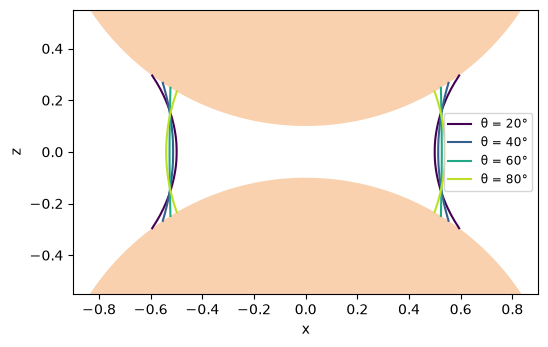
Profiles for several contact angles

The more the liquid wets the beads, the further it spreads over them and the narrower its neck. Cross-sections through the plane \(y = 0\):

def profile(ev):
    # (x, z) where the liquid surface crosses the half-plane y = 0, x > 0
    curve = max(ev.mesh().slice((0, 1, 0)), key=lambda c: c[:, 0].mean())
    return curve[:, 0], curve[:, 2]

fig, ax = plt.subplots(figsize=(6, 4))
c = 1 + gap/2
s = np.linspace(0, 2*np.pi, 200)
for z in (-c, c):
    ax.fill(np.cos(s), z + np.sin(s), color="sandybrown", alpha=0.5, lw=0)
for th, color in zip((20, 40, 60, 80), plt.cm.viridis(np.linspace(0, 0.9, 4))):
    x, z = profile(liquid_bridge(gap, th, volume))
    ax.plot(x, z, color=color, label=f"θ = {th}°")
    ax.plot(-x, z, color=color)
ax.set_aspect("equal")
ax.set_xlim(-0.9, 0.9)
ax.set_ylim(-0.55, 0.55)
ax.set_xlabel("x")
ax.set_ylabel("z")
ax.legend(loc="center right", fontsize="small");

Force against gap

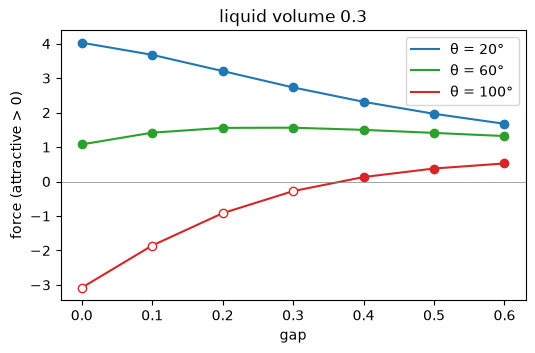
Wetting liquids pull the beads together, the more strongly the smaller the contact angle. Non-wetting liquids (\(\theta \gtrsim 90°\)) push them apart at small gaps, but there the symmetric bridge is unstable: the Hessian has a pair of negative eigenvalues, sideways shifts in \(x\) and \(y\), so the drop would rather slide out of the gap. Such points are drawn hollow. (Each point is a fresh bridge, about half a second each.)

import warnings

gaps = np.linspace(0.0, 0.6, 7)
fig, ax = plt.subplots(figsize=(6, 3.5))
for th, color in zip((20, 60, 100), ("tab:blue", "tab:green", "tab:red")):
    forces, stable = [], []
    for g in gaps:
        with warnings.catch_warnings():   # the unstable bridges: see above
            warnings.simplefilter("ignore", pyse.UnstableEquilibriumWarning)
            b = liquid_bridge(g, th, volume)
        # every Evolver is a handle to the one engine: use b before the next build
        forces.append(force(b))
        stable.append(b.eigen_counts().negative == 0)
    forces, stable = np.array(forces), np.array(stable)
    ax.plot(gaps, forces, "-", color=color, label=f"θ = {th}°")
    ax.plot(gaps[stable], forces[stable], "o", color=color)
    ax.plot(gaps[~stable], forces[~stable], "o", mfc="white", color=color)
ax.axhline(0, color="gray", lw=0.5)
ax.set_xlabel("gap")
ax.set_ylabel("force (attractive > 0)")
ax.set_title(f"liquid volume {volume}")
ax.legend();

How far a bridge stretches

Pull the beads apart and a bridge of fixed volume breaks at some gap. The beads follow the parameter gap, so recipes.arclength can pull them, as on the bridge page it shrinks the liquid, until the bridge’s first unstable mode. What ends the symmetric bridge is one of two things. At its fold no symmetric bridge of that volume spans a wider gap: the neck thins and pinches in the middle. Or, before that, at a branch point, bridges whose neck sits off the mid-plane branch off and the symmetric one turns unstable: the liquid moves toward one bead. The exact axisymmetric bridges (stress_helpers.py, as on the bridge page) say which comes first: here, the volume that breaks at gaps 0.4 and 0.7. Pulling a bridge of that volume apart should then break it at that gap.

A rule widely used in simulations of wet granular matter is the rupture distance of Lian, Thornton and Adams, \(s_c \approx (1 + \theta/2)\,V^{1/3}\) (\(\theta\) in radians, lengths in bead radii).

from pysurfaceevolver import recipes
from stress_helpers import bridge_spheres_branch, bridge_spheres_fold

def breaking_volume(gap, theta):
    # the least volume a stable symmetric bridge holds at this gap (exact), and why
    necks = (0.005, 0.6)
    fold = bridge_spheres_fold(gap, theta, necks=necks)
    try:
        branch = bridge_spheres_branch(gap, theta, necks=necks)
    except ValueError:
        branch = None
    if branch is not None and branch["neck"] > fold["neck"]:
        return branch["volume"], "branch point"
    return fold["volume"], "fold"

results = {}
for th in (20.0, 60.0):
    for g in (0.4, 0.7):
        v, why = breaking_volume(g, th)
        # a bridge of that volume at a gap 0.07 narrower (built the usual way and
        # shrunk to it), pulled apart until it turns unstable
        b = liquid_bridge(g - 0.07, th, 0.15)
        stable = None
        with warnings.catch_warnings():
            warnings.simplefilter("ignore", pyse.UnstableEquilibriumWarning)
            for step in recipes.continuation(b, b.body(1), np.geomspace(0.15, v, 8)[1:]):
                pass
            for step in recipes.arclength(b, "gap", 0.01, 60):
                if step.result.negative_modes:
                    break
                stable = step.value                 # the widest stable gap so far
        lian = (1 + np.radians(th)/2)*v**(1/3)
        results[th, g] = stable, v
        print(f"θ = {th:.0f}°, volume {v:.4f}: stable up to gap {stable:.3f} "
              f"(exact {g}, at the {why}); Lian et al. {lian:.3f}")

fig, ax = plt.subplots(figsize=(6, 3.5))
vs = np.geomspace(0.01, 0.3, 100)
for th, color in ((20.0, "tab:blue"), (60.0, "tab:red")):
    ax.plot(vs, (1 + np.radians(th)/2)*vs**(1/3), color=color, lw=1, label=f"Lian et al., θ = {th:.0f}°")
    for g in (0.4, 0.7):
        stable, v = results[th, g]
        ax.plot(v, g, "o", mfc="white", color=color)
        ax.plot(v, stable, ".", color=color)
ax.set_xscale("log")
ax.set_xlabel("liquid volume")
ax.set_ylabel("gap at which the bridge breaks")
ax.set_title("open: exact; dots: Evolver's widest stable bridge", fontsize="small")
ax.legend(fontsize="small");

/opt/hostedtoolcache/Python/3.12.15/x64/lib/python3.12/site-packages/pysurfaceevolver/_relax.py:658: EvolverWarning: WARNING 1825: Hessian not positive definite. Index: 62
  output.append(self.command(kind))

/tmp/ipykernel_4300/3493961706.py:28: UserWarning: arclength(): no equilibrium found past 0.39849 (even with steps of 0.000156); the surface is back at the last point
  for step in recipes.arclength(b, "gap", 0.01, 60):

θ = 20°, volume 0.0390: stable up to gap 0.398 (exact 0.4, at the fold); Lian et al. 0.398

θ = 20°, volume 0.1848: stable up to gap 0.698 (exact 0.7, at the fold); Lian et al. 0.669

θ = 60°, volume 0.0204: stable up to gap 0.398 (exact 0.4, at the branch point); Lian et al. 0.416

θ = 60°, volume 0.1027: stable up to gap 0.699 (exact 0.7, at the branch point); Lian et al. 0.714

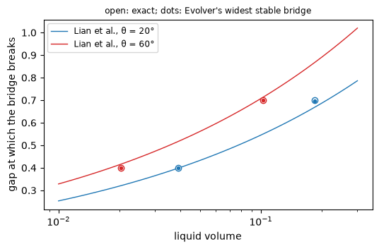
At 20° the bridge reaches its fold: the neck pinches in the middle, and arclength turns back there. At 60° the branch point comes first, well before the fold (at gap 0.4 the fold is at volume 0.0136), and the liquid would go to one bead. Evolver’s widest stable bridge is within 0.01 of the exact gap (the step), on a mesh of about 6000 facets. Lian et al.’s rule gives the gap to within 5% in all four, without telling the two ways of breaking apart.

Exporting for finite elements

For a simulation of the liquid (flow inside the bridge, say), the liquid region needs a closed surface and a volume mesh. Evolver’s mesh is only the liquid–gas interface: the wetted parts of the beads are integrals, not facets, so the body’s surface has two openings. body_surfaces(cap=True) closes each opening with a cap on the constraint its rim lies on (Evolver projects the cap’s points, so this works for any constraint formula), and tells the caps apart.

Every Evolver object is a handle to the one engine, and the sweep above left its last bridge there; build the one to export again:

ev = liquid_bridge(gap, theta, volume)
surface = ev.body_surfaces(cap=True)[1]          # body 1, the liquid

area = surface.areas()                           # the liquid-gas surface, cap 1, cap 2
print("watertight:", surface.watertight, "| caps on constraints:", surface.cap_constraints)
print(f"enclosed volume {surface.volume:.5f} (target {volume})")
print(f"liquid-gas area {area[0]:.5f} (Evolver {ev.total_area:.5f}), "
      f"wetted areas {area[1]:.4f}, {area[2]:.4f}")

watertight: True | caps on constraints: {1: 1, 2: 2}
enclosed volume 0.30008 (target 0.3)
liquid-gas area 1.79212 (Evolver 1.79212), wetted areas 1.0477, 1.0477

volume_mesh fills the closed surface with tetrahedra using Gmsh (pip install gmsh), keeping the surface triangles as they are. The physical groups: 1 for the liquid–gas facets, 2 and 3 for the caps (cap 1 and 2), and the body id for the tetrahedra. A .msh path keeps the group names; that is what dolfinx.io.gmshio.read_from_msh reads.

import os, tempfile
import meshio

folder = tempfile.mkdtemp()
mesh = surface.volume_mesh(size=0.04, path=os.path.join(folder, "bridge.msh"))

tets, P = mesh.cells_dict["tetra"], mesh.points
v = np.einsum("ij,ij->i", P[tets[:, 1]] - P[tets[:, 0]],
              np.cross(P[tets[:, 2]] - P[tets[:, 0]], P[tets[:, 3]] - P[tets[:, 0]]))
print(f"{len(tets)} tetrahedra, volume {np.abs(v).sum()/6:.5f}")
groups = mesh.cell_data_dict["gmsh:physical"]
print("boundary triangles per group:", dict(zip(*np.unique(groups["triangle"], return_counts=True))))

32288 tetrahedra, volume 0.30008
boundary triangles per group: {np.int64(1): np.int64(6144), np.int64(2): np.int64(1536), np.int64(3): np.int64(1536)}

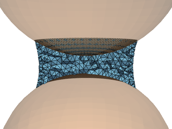
For other FEM codes, meshio writes the tetrahedra and the tagged boundary triangles separately, for example as XDMF:

meshio.write(os.path.join(folder, "bridge.xdmf"),
             meshio.Mesh(P, [("tetra", tets)], cell_data={"region": [groups["tetra"]]}))
meshio.write(os.path.join(folder, "bridge_boundary.xdmf"),
             meshio.Mesh(P, [("triangle", mesh.cells_dict["triangle"])],
                         cell_data={"boundary": [groups["triangle"]]}))
print(sorted(f for f in os.listdir(folder)))

# a cut through the tetrahedra
grid = pv.from_meshio(meshio.Mesh(P, [("tetra", tets)]))
plotter = pv.Plotter()
plotter.add_mesh(grid.clip(normal="y", invert=False, crinkle=True), color="lightskyblue",
                 show_edges=True)
for zc in (-1 - gap/2, 1 + gap/2):
    plotter.add_mesh(pv.Sphere(radius=1.0, center=(0, 0, zc)), color="sandybrown", opacity=0.3)
plotter.camera_position = [(0, -2.6, 0.4), (0, 0, 0), (0, 0, 1)]
plotter.show()

['bridge.h5', 'bridge.msh', 'bridge.xdmf', 'bridge_boundary.h5', 'bridge_boundary.xdmf']

Notes and limits

• Changing parameters on a relaxed bridge. ev.parameters["theta"] = ... (or "gap") followed by ev.relax() works for small changes and for lowering the contact angle; large jumps, or raising the angle so that the contact line has to retreat, can leave folded facets at the contact line (the energy is still right, but the measured angle is not). liquid_bridge(...) builds afresh each time, which takes about half a second.

• Stability. A relaxed bridge is an equilibrium, not necessarily a stable one: check ev.eigen_counts().negative. Non-wetting bridges at small gaps are saddles (see above).

• Rupture. Past the volumes and gaps of how far a bridge stretches a bridge is unstable and would break; the mesh cannot follow a pinch-off, so relaxing fails there (for example volume 0.05 at gap 0.5).

• Unequal beads, gravity, … follow the same pattern: another sphere radius or centre in the constraint formulas, Body(volume=..., density=...) and ev.gravity.

Further reading

• G. Lian, C. Thornton and M. Adams, A theoretical study of the liquid bridge forces between two rigid spherical bodies, J. Colloid Interface Sci. 161 (1993) 138–147, doi:10.1006/jcis.1993.1452. The rupture distance used above.

A bridge between two beads is the smallest liquid structure in a wet bead pack. With more liquid, neighbouring bridges merge into clusters that wet three or more beads. Surface Evolver has computed these shapes in:

• M. Scheel, R. Seemann, M. Brinkmann, M. Di Michiel, A. Sheppard, B. Breidenbach and S. Herminghaus, Morphological clues to wet granular pile stability, Nature Materials 7 (2008) 189–193, doi:10.1038/nmat2117. X-ray tomography of wet bead packs, with bridges, trimers, pentamers and filled tetrahedra computed in Surface Evolver: the pack’s cohesion barely depends on the amount of liquid.

• C. Semprebon, M. Scheel, S. Herminghaus, R. Seemann and M. Brinkmann, Liquid morphologies and capillary forces between three spherical beads, Phys. Rev. E 94 (2016) 012907, doi:10.1103/PhysRevE.94.012907. Two or three merged bridges between three beads: their shapes, forces and stability limits.

• J. Wang, E. Gallo, B. François, F. Gabrieli and P. Lambert, Capillary force and rupture of funicular liquid bridges between three spherical bodies, Powder Technology 305 (2017) 89–98, doi:10.1016/j.powtec.2016.09.060. The force and rupture of liquid between three spheres pulled apart.

• K. Melnikov, R. Mani, F. K. Wittel, M. Thielmann and H. J. Herrmann, Grain-scale modeling of arbitrary fluid saturation in random packings, Phys. Rev. E 92 (2015) 022206, doi:10.1103/PhysRevE.92.022206. A model of whole random packings, from dry to saturated, that takes its bridges’ pressure and volume from Semprebon et al.’s Surface Evolver tables.

Next

Solder joints computes forces with ev.derivative (for a parameter that moves a pad) and lets a loaded chip find its own height. The slit droplet puts a liquid against several walls and mirror planes at once. More drops against walls, from Brakke’s datafiles: drops and capillarity.