Tutorial: a double bubble, from arrays to FEM mesh

Two bubbles of volume 1 and 2 share a film. Surface tension pulls the films toward minimal total area while the volumes stay fixed: the result is the standard double bubble, three spherical caps meeting at 120° along a circle. This notebook builds that surface from arrays, relaxes it, refines the answer with high-order (Lagrange) elements, plots it, and exports watertight surfaces per bubble for a finite-element mesher. It assumes the drop on a table and the conventions of Getting started.

In Jupyter, use pv.set_jupyter_backend("trame") (installed with pip install "pysurfaceevolver[jupyter]") for interactive 3D views; these docs draw static images.

import numpy as np
import pyvista as pv
import pysurfaceevolver as pyse
from pysurfaceevolver import Body, Evolver

pv.set_jupyter_backend("static")
pv.global_theme.window_size = [600, 400]

1. Build the starting surface

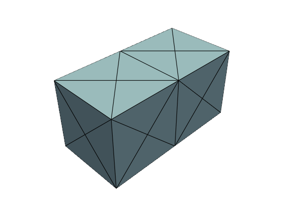
Start from two unit cubes side by side: body 1 is \(x \in [0, 1]\), body 2 is \(x \in [1, 2]\), and the square at \(x = 1\) is their shared film. Faces are vertex loops, in any order around the square; each body lists its faces. When a body’s faces close a surface, as here, load_arrays orients them outward itself (otherwise give orientation: +1 or -1 per face, whether the face’s normal by its vertex order points out of the body).

vertices = np.array([(x, y, z) for x in (0, 1, 2) for y in (0, 1) for z in (0, 1)], float)

def square(axis, value, xmin=0, xmax=2):
    # the face {coordinate `axis` = value} within xmin <= x <= xmax, as a loop
    rows = [i for i, v in enumerate(vertices) if v[axis] == value and xmin <= v[0] <= xmax]
    a, b = [k for k in range(3) if k != axis]
    center = vertices[rows].mean(axis=0)
    angle = np.arctan2(vertices[rows, b] - center[b], vertices[rows, a] - center[a])
    return [rows[i] for i in np.argsort(angle)]

faces = [square(0, 0), square(0, 1), square(0, 2)]          # the film between: faces[1]
for lo, hi in ((0, 1), (1, 2)):
    faces += [square(axis, value, lo, hi) for axis in (1, 2) for value in (0, 1)]

bodies = [Body(faces=[0, 1, 3, 4, 5, 6], volume=1.0),
          Body(faces=[1, 2, 7, 8, 9, 10], volume=2.0)]
ev = Evolver()
ev.load_arrays(vertices, faces, bodies=bodies)
ev

Evolver

datafile	surface.fe
model	soapfilm, linear
elements	23 vertices · 64 edges · 44 facets · 2 bodies
energy	11
area	11
threads	1 · solver evolver

Bodies

body	volume	target	pressure
1	1	1	0	fixed
2	1	2	0	fixed

Evolver triangulated the squares (each got a center vertex). Body 2 starts with volume 1 but its target is 2, so the first iterations inflate it.

ev.plot(color="lightblue")

2. Relax

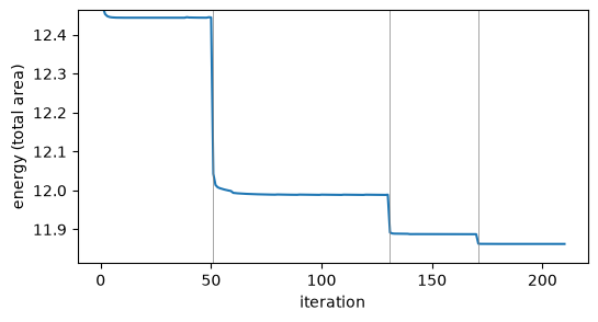
iterate takes gradient-descent steps. relax brings the surface to an equilibrium: gradient steps that keep the mesh in shape, then Newton steps, until the remaining force imbalance (ev.residual()) is small. It also checks that the equilibrium is stable, and warns if it isn’t. levels=3 refines and relaxes again three times: refining in steps, relaxing after each, keeps the surface close to equilibrium. Relaxing a surface says what relax() does on the way. Without walls, ev.energy is simply the total area.

history = [ev.iterate(30)]
result = ev.relax(levels=3)
history.append(result)
print(f"{ev.counts['facets']} facets, energy {ev.energy:.10f}, converged {result.converged} "
      f"(residual {result.residual:.1e}), {result.newton_steps} Newton steps, stable {result.stable}")

2816 facets, energy 11.8626007118, converged True (residual 8.3e-10), 3 Newton steps, stable True

import matplotlib.pyplot as plt

energy = np.concatenate([h.energy for h in history])
fig, ax = plt.subplots(figsize=(6, 3))
ax.plot(energy)
ax.set_xlabel("iteration")
ax.set_ylabel("energy (total area)")
offset = len(history[0].energy)
for s in offset + np.flatnonzero(np.diff(result.level)) + 1:
    ax.axvline(s, color="gray", lw=0.5)    # refinements
ax.set_ylim(energy[-1] - 0.05, energy[-1] + 0.6);

The volume constraints have Lagrange multipliers: the bubbles’ pressures. By the Young–Laplace law the pressure jump across a film is twice its mean curvature (the energy is area, so the tension is 1): the outer films have mean curvature \(p_i/2\), and the shared film \((p_1 - p_2)/2\). The smaller bubble has the higher pressure, so the shared film bulges into the larger one.

ev.bodies()

Bodies

body	volume	target	pressure
1	1	1	2.969907041	fixed
2	2	2	2.469226421	fixed

mesh = ev.mesh()
shared = (mesh.facet_bodies > 0).all(axis=1)          # films with a body on both sides
H = ev.values("vertex", "mean_curvature")
p1, p2 = ev.bodies().pressure
print(f"pressures {p1:.4f}, {p2:.4f}: mean curvatures p1/2 = {p1/2:.4f}, "
      f"p2/2 = {p2/2:.4f}, (p1 - p2)/2 = {(p1 - p2)/2:.4f}")
# the shared film sits inside: draw the outer films translucent
poly = mesh.to_pyvista(point_values={"mean curvature": H})
plotter = pv.Plotter()
style = dict(scalars="mean curvature", clim=[0, 1.6], cmap="viridis")
plotter.add_mesh(poly.extract_cells(np.flatnonzero(~shared)), opacity=0.5, **style)
plotter.add_mesh(poly.extract_cells(np.flatnonzero(shared)), show_edges=True, **style)
plotter.show()

pressures 2.9699, 2.4692: mean curvatures p1/2 = 1.4850, p2/2 = 1.2346, (p1 - p2)/2 = 0.2503

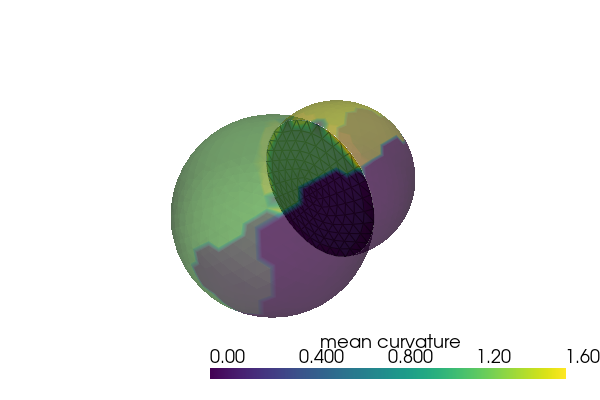
The colors show the three caps of constant mean curvature; the shared film, drawn opaque, is the flattest. (Vertices on the triple junction, where three films meet, have no meaningful mean curvature.) A live view redraws while a run goes on; in Jupyter with the trame backend it updates in place:

view = ev.live_view("area")
ev.iterate(200, callback=view.update, every=10)

3. High-order final stage

The linear model approximates each cap by flat triangles, so the area converges only as the mesh is refined. Once the triangulation is settled, Lagrange elements of order \(n\) give much more accurate energies on the same mesh. In those models relax() does what Brakke’s manual recommends, five gradient steps and then Newton steps. Compare with one more linear refinement:

settled = ev.save()                       # the linear equilibrium
linear = {ev.counts["facets"]: ev.energy}
ev.refine(); ev.relax()
linear[ev.counts["facets"]] = ev.energy

ev.restore(settled)
lagrange = {}
for order in (2, 3, 4):
    ev.set_model("lagrange", order)
    ev.relax()
    lagrange[order] = ev.energy

coarse = min(linear)
for facets, e in linear.items():
    print(f"linear      {facets:6d} facets  energy {e:.12f}")
for order, e in lagrange.items():
    print(f"Lagrange {order}  {coarse:6d} facets  energy {e:.12f}")

linear        2816 facets  energy 11.862600711800
linear       11264 facets  energy 11.856368562986
Lagrange 2    2816 facets  energy 11.854293307045
Lagrange 3    2816 facets  energy 11.854293130575
Lagrange 4    2816 facets  energy 11.854293128000

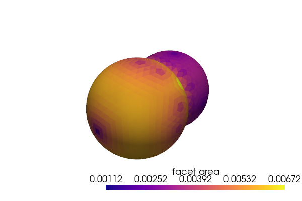
Lagrange 3 on the coarser mesh already agrees with Lagrange 4 to about a few \(10^{-9}\), far better than the linear model on four times as many facets. Plots and exports sample the curved facets; the facet sizes still show where the cube’s corners were:

ev.plot("area", n=4, show_edges=False, cmap="plasma",
        scalar_bar_args={"title": "facet area"})

4. Export for finite elements

body_surfaces gives each bubble’s closed surface with outward normals (the shared film belongs to both). write_bodies writes one file per body, either as flat triangles sampled on the curved facets (curved="tessellate") or as native high-order triangles (curved="native"; Gmsh format, here quadratic since Gmsh meshers take order-2 surfaces).

for s in ev.body_surfaces(n=4).values():
    print(f"body {s.body}: {len(s.cells)} triangles, watertight {s.watertight}")

body 1: 24576 triangles, watertight True
body 2: 24576 triangles, watertight True

import os, tempfile
import meshio

out = tempfile.mkdtemp()
ev.write_bodies(os.path.join(out, "bubble_{id}.stl"), n=4)

ev.set_model("lagrange", 2)
ev.relax()
ev.write_bodies(os.path.join(out, "bubble_{id}.msh"), curved="native")
print(sorted(os.listdir(out)))

def enclosed_volume(points, triangles):
    a, b, c = (points[triangles[:, i]] for i in range(3))
    return np.einsum("ij,ij->i", a, np.cross(b, c)).sum() / 6

import warnings
warnings.filterwarnings("ignore", "overflow", RuntimeWarning)   # meshio's STL reader

for body in (1, 2):
    stl = meshio.read(os.path.join(out, f"bubble_{body}.stl"))
    msh = meshio.read(os.path.join(out, f"bubble_{body}.msh"))
    tris = stl.cells_dict["triangle"]
    print(f"body {body}: STL volume {enclosed_volume(stl.points, tris):.6f}; "
          f".msh cells {[(c.type, len(c.data)) for c in msh.cells]}")

['bubble_1.msh', 'bubble_1.stl', 'bubble_2.msh', 'bubble_2.stl']

body 1: STL volume 0.999645; .msh cells [('triangle6', 1536)]

body 2: STL volume 1.999214; .msh cells [('triangle6', 1536)]

The flat triangles enclose the target volumes to within 0.05% (the curved surface is sampled at their corners); the .msh files hold quadratic triangles (triangle6) with the facet ids as Gmsh physical and geometrical tags, ready for a volume mesher.

Next

• Relaxing a surface explains what relax() did here, how to read its result, and where its defaults stop working.

• The liquid bridge adds walls: a drop between two beads, with contact angles, forces and a volume mesh.

• ev.command(...) runs any Evolver command; the manual describes them all. pyse.map runs parameter sweeps in worker processes, one engine each. The API reference documents every public class and function.